SmoothlyBrokenPowerLaw1D
-
class
astropy.modeling.powerlaws.SmoothlyBrokenPowerLaw1D(amplitude=1, x_break=1, alpha_1=-2, alpha_2=2, delta=1, **kwargs)[source] [edit on github]¶ Bases:
astropy.modeling.Fittable1DModelOne dimensional smoothly broken power law model.
Parameters: amplitude : float
Model amplitude at the break point.
x_break : float
Break point.
alpha_1 : float
Power law index for
x << x_break.alpha_2 : float
Power law index for
x >> x_break.delta : float
Smoothness parameter.
See also
Notes
Model formula (with
 for
for amplitude, for
for
x_break, for
for alpha_1, for
for alpha_2and for
for
delta):![f(x) = A \left( \frac{x}{x_b} \right) ^ {-\alpha_1}
\left\{
\frac{1}{2}
\left[
1 + \left( \frac{x}{x_b}\right)^{1 / \Delta}
\right]
\right\}^{(\alpha_1 - \alpha_2) \Delta}](../_images/math/cab0fc27bc5f994e2638f3b21bb3b7f77500f025.png)
The change of slope occurs between the values
 and
and  such that:
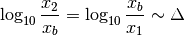
At values
 and
and  the
model is approximately a simple power law with index
and respectively. The two
power laws are smoothly joined at values
the
model is approximately a simple power law with index
and respectively. The two
power laws are smoothly joined at values  ,
hence the parameter sets the “smoothness” of the
slope change.
,
hence the parameter sets the “smoothness” of the
slope change.The
deltaparameter is bounded to values greater than 1e-3 (corresponding to ) to avoid
overflow errors.
) to avoid
overflow errors.The
amplitudeparameter is bounded to positive values since this model is typically used to represent positive quantities.Examples
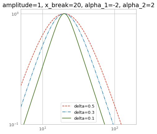
import numpy as np
import matplotlib.pyplot as plt
from astropy.modeling import models

x = np.logspace(0.7, 2.3, 500)
f = models.SmoothlyBrokenPowerLaw1D(amplitude=1, x_break=20,
                                    alpha_1=-2, alpha_2=2)

plt.figure()
plt.title("amplitude=1, x_break=20, alpha_1=-2, alpha_2=2")

f.delta = 0.5
plt.loglog(x, f(x), '--', label='delta=0.5')

f.delta = 0.3
plt.loglog(x, f(x), '-.', label='delta=0.3')

f.delta = 0.1
plt.loglog(x, f(x), label='delta=0.1')

plt.axis([x.min(), x.max(), 0.1, 1.1])
plt.legend(loc='lower center')
plt.grid(True)
plt.show()
Attributes Summary
alpha_1alpha_2amplitudedeltainput_unitsparam_namesx_breakMethods Summary
evaluate(x, amplitude, x_break, alpha_1, ...)One dimensional smoothly broken power law model function fit_deriv(x, amplitude, x_break, alpha_1, ...)One dimensional smoothly broken power law derivative with respect Attributes Documentation
-
alpha_1
-
alpha_2
-
amplitude
-
delta
-
input_units
-
param_names= ('amplitude', 'x_break', 'alpha_1', 'alpha_2', 'delta')
-
x_break
Methods Documentation
-
static
evaluate(x, amplitude, x_break, alpha_1, alpha_2, delta)[source] [edit on github]¶ One dimensional smoothly broken power law model function
-
static
fit_deriv(x, amplitude, x_break, alpha_1, alpha_2, delta)[source] [edit on github]¶ One dimensional smoothly broken power law derivative with respect to parameters
-