Analysis¶

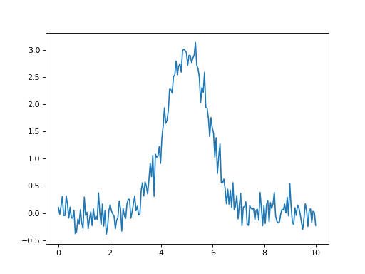
The specutils package comes with a set of tools for doing common analysis tasks on astronomical spectra. Some examples of applying these tools are described below. The basic spectrum shown here is used in the examples in the sub-sections below - see Working with Spectrum1Ds for more on creating spectra:

>>> import numpy as np
>>> from astropy import units as u
>>> from astropy.nddata import StdDevUncertainty
>>> from astropy.modeling import models
>>> from specutils import Spectrum1D, SpectralRegion
>>> np.random.seed(42)
>>> spectral_axis = np.linspace(0., 10., 200) * u.GHz
>>> spectral_model = models.Gaussian1D(amplitude=3*u.Jy, mean=5*u.GHz, stddev=0.8*u.GHz)
>>> flux = spectral_model(spectral_axis)
>>> flux += np.random.normal(0., 0.2, spectral_axis.shape) * u.Jy
>>> uncertainty = StdDevUncertainty(0.2*np.ones(flux.shape)*u.Jy)
>>> noisy_gaussian = Spectrum1D(spectral_axis=spectral_axis, flux=flux, uncertainty=uncertainty)
>>> import matplotlib.pyplot as plt 
>>> plt.plot(noisy_gaussian.spectral_axis, noisy_gaussian.flux) 

(Source code, png, hires.png, pdf)

SNR¶

The signal-to-noise ratio of a spectrum is often a valuable quantity for evaluating the quality of a spectrum. The specutils.analysis.snr function performs this task, either on the spectrum as a whole, or sub-regions of a spectrum:

>>> from specutils.analysis import snr
>>> snr(noisy_gaussian)  
<Quantity 2.95214319>
>>> snr(noisy_gaussian, SpectralRegion(4*u.GHz, 6*u.GHz))  
<Quantity 11.84806008>

Line Flux Estimates¶

While line-fitting (see Line/Spectrum Fitting) is a more thorough way to measure spectral line fluxes, direct measures of line flux are very useful for either quick-look settings or for spectra not amedable to fitting. The specutils.analysis.line_flux function addresses that use case. The closely related specutils.analysis.equivalent_width computes the equivalent width of a spectral feature, a flux measure that is normalized against the continuum of a spectrum. Both are demonstrated below:

Note

The specutils.analysis.line_flux function assumes the spectrum has already been continuum-subtracted, while specutils.analysis.equivalent_width assumes the continuum is at a fixed, known level (defaulting to 1, meaning continuum-normalized). Continuum Fitting describes how continuua can be generated to prepare a spectrum for use with these functions.

>>> from specutils.analysis import line_flux
>>> line_flux(noisy_gaussian).to(u.erg * u.cm**-2 * u.s**-1)  
<Quantity 5.92896407e-14 erg / (cm2 s)>
>>> #line_flux(noisy_gaussian, SpectralRegion(3*u.GHz, 7*u.GHz))  
<Quantity 6e-14 erg / (cm2 s)>

For the equivalen width, note the need to add a continuum level:

>>> from specutils.analysis import equivalent_width
>>> noisy_gaussian_with_continuum = noisy_gaussian + 1*u.Jy
>>> equivalent_width(noisy_gaussian)  
<Quantity 4.07103593 GHz>
>>> equivalent_width(noisy_gaussian, SpectralRegion(3*u.GHz, 7*u.GHz))  
<Quantity -5 GHz>

Centroid¶

The specutils.analysis.centroid function provides a first-moment analysis to estimate the center of a spectral feature:

>>> from specutils.analysis import centroid
>>> centroid(noisy_gaussian, SpectralRegion(3*u.GHz, 7*u.GHz))  
<Quantity 4.99604264 GHz>

While this example is “pre-subtracted”, this function only performs well if the contiuum has already been subtracted, as for the other functions above and below.

Line Widths¶

There are several width statistics that are provided by the specutils.analysis submodule.

The gaussian_sigma_width function estimates the width of the spectrum by computing a second-moment-based approximation of the standard deviation.

The gaussian_fwhm function estimates the width of the spectrum at half max, again by computing an approximation of the standard deviation.

Both of these functions assume that spectrum is approximately gaussian.

The function fwhm provides an estimate of the full width of the spectrum at half max that does not assume the spectrum is gaussian. It locates the maximum, and then locates the value closest to half of the maximum on either side, and measures the distance between them.

Each of the width analysis functions are applied to this spectrum below:

>>> from specutils.analysis import gaussian_sigma_width, gaussian_fwhm, fwhm
>>> gaussian_sigma_width(noisy_gaussian) 
<Quantity 0.93853592 GHz>
>>> gaussian_fwhm(noisy_gaussian) 
<Quantity 2.21008321 GHz>
>>> fwhm(noisy_gaussian) 
<Quantity 1.65829146 GHz>

Reference/API¶

Functions¶

`centroid`(spectrum, region)	Calculate the centroid of a region, or regions, of the spectrum.
`equivalent_width`(spectrum[, continuum, regions])	Computes the equivalent width of a region of the spectrum.
`fwhm`(spectrum[, region])	Compute the true full width half max of the spectrum.
`gaussian_fwhm`(spectrum[, region])	Estimate the width of the spectrum using a second-moment analysis.
`gaussian_sigma_width`(spectrum[, region])	Estimate the width of the spectrum using a second-moment analysis.
`line_flux`(spectrum[, regions])	Computes the integrated flux in a spectrum or region of a spectrum.
`snr`(spectrum[, region])	Calculate the mean S/N of the spectrum based on the flux and uncertainty in the spectrum.

Navigation